Executive summary:

I used supervised and unsupervised machine learning algorithms—primarily Multiple Linear Regression, Principle Component Analysis, and Clustering—to accurately predict prices for Sberbank’s Russian Housing Market Kaggle competition. I developed these models using a data pipeline that cleaned the data based on my research findings, tidied the data into Third Normal Form, transformed features to appropriately fit the models used, engineered new features where appropriate, imputed missing data using K-Nearest Neighbors. I then used the Bayes Information Criterion and residual plots to identify important and sensible underlying factors that affect housing prices, and I created a predictive model with validation.

 

Motivations:

My first glance into the world of Kaggle competitions was an interesting one: international sanctions, a collapsing oil economy, a nascent coffee culture, and tax fraud all contributed significantly to a proper understanding of Sberbank’s Moscow housing market dataset. As a business-facing problem, successful analysis of such a dataset must include two main components: insights brought forth by interpretation of the data, and accurate predictions brought forth by the best model. Below I present how to go about this tall task and a review of the major factors that impact the nominal price of housing in Moscow.

 

The objective of this competition was to accurately predict prices of housing units in Moscow for Sberbank given the data it provided on Kaggle. This included a set of macroeconomic data from the years 2010-2016 (overlapping Russia’s conflict in Crimea and its international response of increasing sanctions, along with the collapse of the Russian oil economy that followed), and a set of housing unit data from the same period, with prices for the period from 2010 to April 2015, and an unpriced test set from April 2015 onward used for model scoring and ranking.

 

Aside from typical issues with missingness and inaccuracy that one expects in any real-world dataset, first attempts at modeling the data performed unsatisfactorily due to an insidious issue with the quality of the data: a predominance of uniformly cheaply-priced units in the far left tail of the price histogram. See below:

This slideshow requires JavaScript.

 

Such effects were further compounded by the fact that the Support Vector Machine I constructed failed to classify which units might end up selling at such a “subsidized” price and which would sell at prices within the typical distribution for Moscow houses. This vexing class of housing units ended up having a much simpler explanation after I briefly looked into Russian capital gains law: tax fraud. It’s apparently common practice to report significantly lower house prices for the purposes of property tax evasion, so I assigned all suspicious prices (the glut of prices clustered at or just below the RUB 1 million and 2 million property tax cut-offs) to missing and imputed instead, which greatly improved the accuracy of the model. Sometimes the answer to a data conundrum comes from outside the data.

 

Additional preliminary looks into the data revealed that Sberbank would strongly benefit from a data engineering team. The dataset Sberbank provided was primarily composed of highly redundant features slapped together into an inconsistent and amorphous blob that violated basic Tidy Data principles in multiple ways. In light of this, I developed a data cleaning and tidying pipeline that was key in my team’s success in the competition. Here are some of the ways I confronted these issues:

 

I set out to build an interpretable multiple linear regression model with the goal of providing useful insights into the Moscow housing market (as opposed to using a more powerful black-box model). I constructed this model using features engineered in three ways: native features transformed to avoid violating requirements for use in a linear regression model (e.g. linearity, homoscedasticity, and a normal-like distribution), composite features generated to avoid issues associated with multilinear regressions (i.e. PCA to resolve collinearity), and novel features engineered to better relate a feature’s effect on price (e.g. thresholding and further transformations).

 

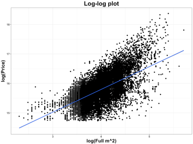
Prices were distributed nearly log-normally (a Box-Cox transformation showed best-fit lambda close to 0), so I log-transformed price figures. Other features (such as apartment size) showed much-closer-to linear fit upon log transformation as well (along with much-closer-to normally distributed errors), so for best incorporation into the multilinear regression, I log-transformed those features as well. These log-log relationships also displayed much lower heteroskedasticity compared to those of the untransformed features, further necessitating the transformation. Other features, particularly temporal economic figures, required separate modeling, as they were duplicated with differing frequencies (e.g. Sberbank copy-pasted weekly-measured figures for each other weekday and copy-pasted monthly-measured features for the rest of the month so that one independent measurement masqueraded as multiple separate observations). See an example of the heteroskedasticity below:

This slideshow requires JavaScript.

 

Matrix correlation plots (below) revealed that the dataset consisted of two sets of mostly highly correlated data. The first set contained many of the most explanatory features, so I selected the most useful of these for use in the model and left the rest out. I reduced dimensionality in the second set through PCA and found a handful of useful features (principle components) that I also added to the model. After investigating the significant principal components (left of the “elbow” in a scree plot) for interpretability in addition to significance, I also included the top 10 PCs from the set of distance features and the top 4 PCs from the set of coffee-related and object count features.

 

I explored reducing the complexity of the raion feature using agglomerative clustering, though the lackluster results of such explorations (in addition to the failure of raion characteristics to model raion residuals of the best model missing the raion feature against the true values) further strengthened my sense that the coefficients of the raion categoricals are more a measure of neighborhood popularity (je ne sais quoi) than anything else. It is reasonable to suppose that factors outside (and unmeasured by) the dataset would also be affecting prices; demographic and cultural information for each raion was limited, and such effects would effectively be captured by a catch-all feature like the raion categorical itself.

So what factors do Muscovites react strongly to when pricing a housing unit, and in what ways?

 

Muscovites like:

• larger units (by far the biggest contributor to price)
• desirable neighborhoods (the second-largest contributor)
• units in better condition
• living in taller buildings
• living on higher floors within those buildings
• expensive coffee in the center city (hipsterism?)
• proportionally larger kitchens
• living closer to parks
• living within walkable distance of a metro station
• living near big shopping areas

 

Muscovites don’t like:

• living too far away from the city center (another major contributor)
• living right by highways
• living right by railroads
• living right by power transmission lines
• living right by oil refineries
• panel or breezeblock construction materials
• old buildings
• buildings with contemporary-style architecture, regardless of age

 

Additionally, they’re willing to pay more for ownership-style apartments than investment-style apartments (or house-buyers may be less savvy than real estate investors).

 

Conclusion:

While Kaggle-style competitions tend to reward black box models, kernel-copying, and hyperparameter-hacking through repeated submissions (submitting models fudged by different amounts until the score happens to improve as a kind of over-fitting), I took it as a way to learn how to better perform regular data science, using only the kinds of models and techniques that I could justify to a supervisor looking for insights. It was outperformed by boosted-tree methods in terms of log-error, but held its own very well against less flexible models (being the best multilinear regression among my bootcamp cohort) and solidly accomplished its objectives of providing actionable insights into how potential house buyers in Moscow make pricing decisions.