Category Archives: machine learning

An Basic Approach to Reinforcement Learning

Executive Summary:

Despite my lack of expertise with the topic, I used this approach to win 3rd place at a Trivago hackathon in NYC on November 11, 2017. The task was to improve Trivago in some way (an incredibly open objective), and most teams, including the one I pitched at led, focused on improving Trivago’s web portal and search listings to help grow Trivago’s market share. My idea was roughly to apply a basic reinforcement learning approach to change the static (non-learning) search result ranking algorithm into one that continuously improves its market segmentation based on user interaction with the site. My proposed algorithm ranks search results according to what has worked the best with demographically similar visitors in the past, along with enough randomness to continue learning (i.e. not get stuck in a local minimum). The Trivago judges mentioned that the general idea is one they’re already developing and that they liked my specific approach, which was a bit different than what they had considered thus far.

Motivations:

It is sensible to assume that everyone prefers better-rated hotels at better prices, but I’d expect some customer segments to be more price-sensitive than others. (Some people will always book the cheapest option; some will always book their favorite regardless of price; and some will carefully deliberate.) I think it’s also sensible to assume that this behavior will, to some extent, track with demographic information such as income. And further, since IP is a proxy for location, and location is a proxy for demographic information like income, Trivago and other similar companies should be able to use such information when ranking listings for users.

I created a multi-dimensional space (numpy’s ndarray being the natural choice) that keeps track of how price-sensitive and discount-sensitive demographic segments are: one dimension for income segments (log transformed), one dimension for age segments, and one dimension as a proof-of-concept placeholder for other segments like gender. A final dimension just divides the space up into price-sensitivity information and discount-sensitivity information, though I conceptualize it as a three- (or n-) dimensional space pointing to a two- (or m-) element vector. Such a system does not rely on particular values of m and n, which can be chosen based on what provides the most useful information (n being the number of demographic information types that are useful, and m being the number of sensitivity-to-hotel-aspect features that are useful). I’ll call this the “demographic preference space”.

I initialize a few parameters, such as the learning rate, the level of randomness, and a set of effect-size parameters that influence how much different types of actions (from greatest to least: creating an account, purchasing through express checkout, clicking on a hotel, or leaving without purchasing anything) affect the demographic preference space. While making a hotel purchase does directly indicate a user liking a particular hotel, there’s unfortunately no direct measure of a user’s dislike of a particular hotel, so I set the effect-size for leaving without purchasing anything as negative to “blame” all the hotels presented to the user a little bit for not being what the user wanted.

Each interaction changes the demographic preference space based on the learning rate and the effect size. When deciding which hotel listings to present to a new user, each hotel that corresponds to their searched terms gets scored based on how that hotel scores along each hotel aspect (price and discount) compared with the assumed preferences of the user based on the demographic preference space. In more detail, a local Gaussian average of price-sensitivity and discount-sensitivity are taken in the demographic preference space, centered at the user’s own demographic position. These sensitivities are passed through a hyperbolic tangent (tanh) function to provide reasonable bounds on their amplitudes. Each sensitivity (for instance, price-sensitivity) is multiplied against its relevant score from the hotel (for instance, price-score), and each of these terms is summed for a total score for the hotel for the user. As I also scaled hotel aspect scores (price scores and discount scores) from +1 to -1, low discount-sensitivity (-1) against low discount (-1) registers as a match, just as high discount-sensitivity (1) against high discount (1). A (relatively small, adjustable) random number is added to the score for each hotel to prevent the algorithm from getting stuck in a local minimum, and the hotels are sorted by score and displayed to the user accordingly.

The main proof of concept was showing that despite initial rankings being random, wealthier and less wealthy phantom users applying their preferences (toward nicer hotels and toward cheaper hotels, respectively) quickly (within a few hundred interactions) resulted in wealthier users being shown accordingly nice hotels and less wealthy users being shown accordingly cheaper hotels.

One major challenge of this competition was the lack of any user or hotel data, which I had to write functions to generate for this proof of concept. That, combined with the competition’s duration of only one day, prevented any more sophisticated approaches, though I had thought of a few. The algorithm as I submitted it does not make any outright assumptions about hotel preferability, instead just following what the users pick. Perhaps a hybrid approach could improve results. There were also plenty of other hotel aspects, most notably rating (and users’ sensitivities to these hotel aspects, e.g. rating-sensitivity), that could have easily been included in the demographic preference space. And despite using some nuts and bolts of neural networks (such as the idea of a learning rate, vaguely convolution-like processing of the demographic preference space, incrementation of weights based on fit/error assessment, and use of functions like tanh to prevent “blowing-up activation”), there was no neural network component to my solution despite being well-suited for such an approach. Had we more time, I would have pursued such low-hanging fruit as next steps.

Predicting House Prices During a Declining Economy: A First Look into Kaggle Competitions

Executive summary:

I used supervised and unsupervised machine learning algorithms—primarily Multiple Linear Regression, Principle Component Analysis, and Clustering—to accurately predict prices for Sberbank’s Russian Housing Market Kaggle competition. I developed these models using a data pipeline that cleaned the data based on my research findings, tidied the data into Third Normal Form, transformed features to appropriately fit the models used, engineered new features where appropriate, imputed missing data using K-Nearest Neighbors. I then used the Bayes Information Criterion and residual plots to identify important and sensible underlying factors that affect housing prices, and I created a predictive model with validation.

Motivations:

My first glance into the world of Kaggle competitions was an interesting one: international sanctions, a collapsing oil economy, a nascent coffee culture, and tax fraud all contributed significantly to a proper understanding of Sberbank’s Moscow housing market dataset. As a business-facing problem, successful analysis of such a dataset must include two main components: insights brought forth by interpretation of the data, and accurate predictions brought forth by the best model. Below I present how to go about this tall task and a review of the major factors that impact the nominal price of housing in Moscow.

The objective of this competition was to accurately predict prices of housing units in Moscow for Sberbank given the data it provided on Kaggle. This included a set of macroeconomic data from the years 2010-2016 (overlapping Russia’s conflict in Crimea and its international response of increasing sanctions, along with the collapse of the Russian oil economy that followed), and a set of housing unit data from the same period, with prices for the period from 2010 to April 2015, and an unpriced test set from April 2015 onward used for model scoring and ranking.

Aside from typical issues with missingness and inaccuracy that one expects in any real-world dataset, first attempts at modeling the data performed unsatisfactorily due to an insidious issue with the quality of the data: a predominance of uniformly cheaply-priced units in the far left tail of the price histogram. See below:

This slideshow requires JavaScript.

Such effects were further compounded by the fact that the Support Vector Machine I constructed failed to classify which units might end up selling at such a “subsidized” price and which would sell at prices within the typical distribution for Moscow houses. This vexing class of housing units ended up having a much simpler explanation after I briefly looked into Russian capital gains law: tax fraud. It’s apparently common practice to report significantly lower house prices for the purposes of property tax evasion, so I assigned all suspicious prices (the glut of prices clustered at or just below the RUB 1 million and 2 million property tax cut-offs) to missing and imputed instead, which greatly improved the accuracy of the model. Sometimes the answer to a data conundrum comes from outside the data.

Additional preliminary looks into the data revealed that Sberbank would strongly benefit from a data engineering team. The dataset Sberbank provided was primarily composed of highly redundant features slapped together into an inconsistent and amorphous blob that violated basic Tidy Data principles in multiple ways. In light of this, I developed a data cleaning and tidying pipeline that was key in my team’s success in the competition. Here are some of the ways I confronted these issues:

I set out to build an interpretable multiple linear regression model with the goal of providing useful insights into the Moscow housing market (as opposed to using a more powerful black-box model). I constructed this model using features engineered in three ways: native features transformed to avoid violating requirements for use in a linear regression model (e.g. linearity, homoscedasticity, and a normal-like distribution), composite features generated to avoid issues associated with multilinear regressions (i.e. PCA to resolve collinearity), and novel features engineered to better relate a feature’s effect on price (e.g. thresholding and further transformations).

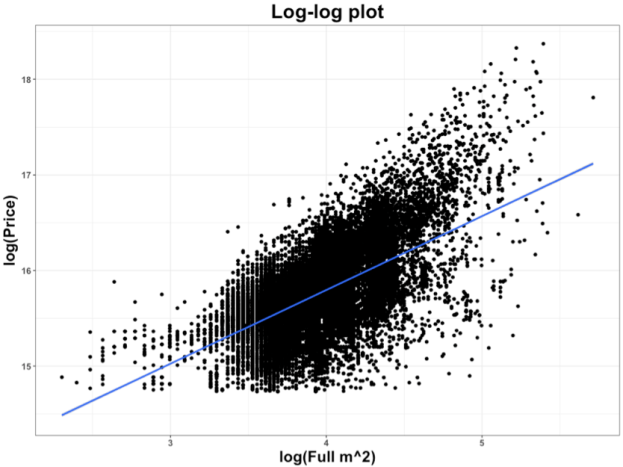
Prices were distributed nearly log-normally (a Box-Cox transformation showed best-fit lambda close to 0), so I log-transformed price figures. Other features (such as apartment size) showed much-closer-to linear fit upon log transformation as well (along with much-closer-to normally distributed errors), so for best incorporation into the multilinear regression, I log-transformed those features as well. These log-log relationships also displayed much lower heteroskedasticity compared to those of the untransformed features, further necessitating the transformation. Other features, particularly temporal economic figures, required separate modeling, as they were duplicated with differing frequencies (e.g. Sberbank copy-pasted weekly-measured figures for each other weekday and copy-pasted monthly-measured features for the rest of the month so that one independent measurement masqueraded as multiple separate observations). See an example of the heteroskedasticity below:

This slideshow requires JavaScript.

Matrix correlation plots (below) revealed that the dataset consisted of two sets of mostly highly correlated data. The first set contained many of the most explanatory features, so I selected the most useful of these for use in the model and left the rest out. I reduced dimensionality in the second set through PCA and found a handful of useful features (principle components) that I also added to the model. After investigating the significant principal components (left of the “elbow” in a scree plot) for interpretability in addition to significance, I also included the top 10 PCs from the set of distance features and the top 4 PCs from the set of coffee-related and object count features.

I explored reducing the complexity of the raion feature using agglomerative clustering, though the lackluster results of such explorations (in addition to the failure of raion characteristics to model raion residuals of the best model missing the raion feature against the true values) further strengthened my sense that the coefficients of the raion categoricals are more a measure of neighborhood popularity (je ne sais quoi) than anything else. It is reasonable to suppose that factors outside (and unmeasured by) the dataset would also be affecting prices; demographic and cultural information for each raion was limited, and such effects would effectively be captured by a catch-all feature like the raion categorical itself.

So what factors do Muscovites react strongly to when pricing a housing unit, and in what ways?

Muscovites like:

larger units (by far the biggest contributor to price)
desirable neighborhoods (the second-largest contributor)
units in better condition
living in taller buildings
living on higher floors within those buildings
expensive coffee in the center city (hipsterism?)
proportionally larger kitchens
living closer to parks
living within walkable distance of a metro station
living near big shopping areas

Muscovites don’t like:

living too far away from the city center (another major contributor)
living right by highways
living right by railroads
living right by power transmission lines
living right by oil refineries
panel or breezeblock construction materials
old buildings
buildings with contemporary-style architecture, regardless of age

Additionally, they’re willing to pay more for ownership-style apartments than investment-style apartments (or house-buyers may be less savvy than real estate investors).

Conclusion:

While Kaggle-style competitions tend to reward black box models, kernel-copying, and hyperparameter-hacking through repeated submissions (submitting models fudged by different amounts until the score happens to improve as a kind of over-fitting), I took it as a way to learn how to better perform regular data science, using only the kinds of models and techniques that I could justify to a supervisor looking for insights. It was outperformed by boosted-tree methods in terms of log-error, but held its own very well against less flexible models (being the best multilinear regression among my bootcamp cohort) and solidly accomplished its objectives of providing actionable insights into how potential house buyers in Moscow make pricing decisions.

“Fake News”: Detecting Bias on Wikipedia using NLP

Executive Summary:

My team partner (Rachel Kogan, a NYC Data Science Academy bootcamp classmate) and I filtered the Wikipedia English corpus down to bags of words using pySpark and trained machine learning models to detect bias (point of view tags) on TF-IDF data with nearly 90% accuracy.

Motivations:

The tide of news about fake news has reached a crescendo, and not many feasible solutions have been proposed for controlling the spread of biased information. The push for Facebook and other large social media sites on which most fake news seems to promulgate to manually editorialize their content is certainly infeasible for one. This problem seems ripe for machine learning approaches, specifically Natural Language Processing, so we set out to develop models that could detect bias in a large textual corpus. Due to its ease of access and pre-labeled content, we trained our models on the English Wikipedia corpus.

Wikipedia is one of the topmost visited websites in the English-speaking world and serves as a first go-to when looking for a quick overview on almost any topic. It’s surprisingly accurate and reliable given its anyone-can-edit ideology and site structure (roughly as reliable as the Encyclopedia Britannica according to a 2005 Nature study). Bots and users alike peruse the site for vandalism and other problematic edits, marking certain sentences, paragraphs, and entire articles as having a problem from a specific set of pre-defined tags. Fortunately for us, POV, or point of view (implying non-neutral point of view) is one such tag. There are several thousand articles in the English language Wikipedia with current POV tags, which provided a substantial enough body of data with which to train a bias detector. We downloaded the entire current-version (as of May 2017) English Wikipedia corpus in XML and stored it in the cloud using Amazon’s EC2 and S3 services. After separating the massive (~64GB) textual dataset into separate pages by the embedded XML page tags, we were able to filter the pages down to the usable articles (removing redirect pages, talk and other user pages, and simple list pages). The POV tags within each page’s text follow a replicable format (“{{POV … }}”), allowing for a regex-like filtering of the total articles down to just the articles with POV issues, and furthermore, articles for which the entire body of text is tagged as having POV issues (as opposed to just a paragraph or single line) also show a replicable special POV tag located in the header of the text, making filtering out articles with only very minor POV issues simple.

We then sampled from the rest of the corpus (presumably without POV issues) to generate training and test data sets with roughly equal proportions of non-neutral and relatively neutral articles. The XML markdown-style documents were then parsed with a set of regular expressions to generate a simple bag of words for each article (thereby removing all tags, including those that mark the article as having POV issues). We tokenized the bags of words and removed stop-words, followed by generating TF-IDF values for each unique term in each document (Term Frequency Inverse Document Frequency is a canonical way to calibrate simple bag of words term counts into relative term importances by adjusting by the rarity of each term across the entire corpus).

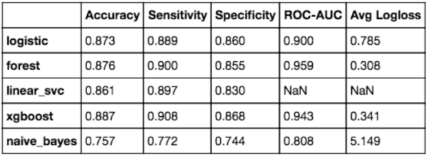
We trained many kinds of models to analyze which may be best at detecting bias in Wikipedia articles (and, by extension, in other sources of textual data as well). Among the best performers were logistic regression, random forest, and XGBoost (see metrics below).

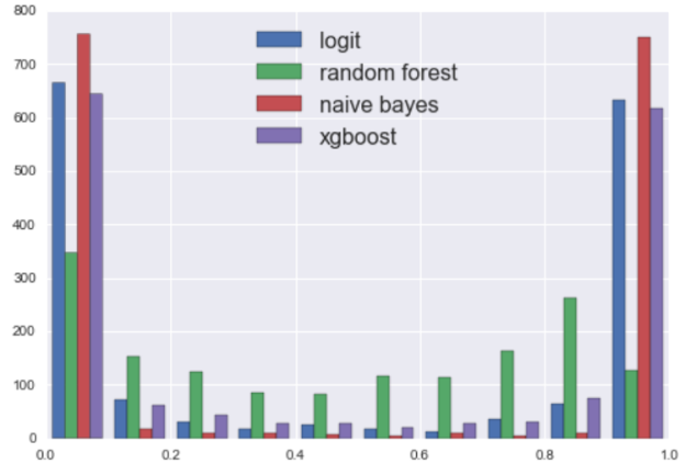
Additionally, we found that our models were fairly confident in their predictions, giving further credence to the idea that something as complicated as bias can be well handled by NLP and machine learning methods (x-axis is predicted probability, and y-axis is the number of such observations):

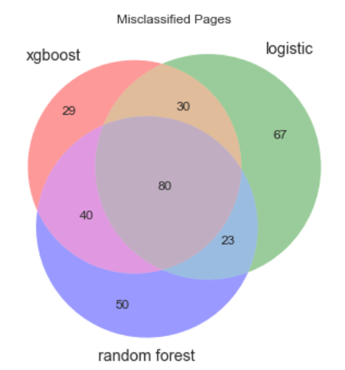
We further investigated correlations in misclassification between these models to see if an ensembled approach would significantly improve our results. However, high correlations between our models limited the extent to which we could improve our overall misclassification rate through ensembling. As you can see below, any majority-voting metric would have misclassified at nearly the same rate.