Category Archives: image analysis

Hidden in Plain Sight: Scraping Amazon Price History Data from Images on the Web

Executive Summary:

Where previous bootcamp students had tried and failed to scrape Amazon for price history data, I succeeded—not by being smarter, but by taking a more creative approach. I instead scraped a third party site that tracks Amazon—CamelCamelCamel—and recreated Amazon price data by analyzing graph images displayed on the site. I didn’t actually scrape Amazon, but I successfully obtained the same data (within a fraction of a percent rounding error) by cross-applying my skills in image analysis in a different domain.


Motivations:

Amazon price data is freely available through the Amazon API, limited at a generous 1 million API calls per month. As a competitor or consumer on the marketplace, price history data are extremely useful and can drive much wiser decisions about when and what to buy and at what price. But seeing the current prices (that’s all they provide) only gives a fraction of the total picture: how do the current prices compare with prices from the recent past? When deciding to purchase or sell a stock or trade in foreign currencies, one would naturally want to look at the price or exchange history. Analogously, what about Amazon price history data? Such historical pricing data were apparently available directly through an Amazon service in the past, but today Amazon does not provide such a service and does not make it possible to scrape such data directly from the Amazon web system, leaving consumers and retailers to search for this information elsewhere. As these price history data are quite valuable, websites do exist that provide access to such information; among these are CamelCamelCamel and Tracktor. (Terapeak allows pinging price history for Amazon items, but at a paltry 500 API calls per month.) These websites make the data available in graphical form only, perfect for letting consumers and retailers quickly and qualitatively improve their decisions to buy or sell at optimal times. By not directly providing the underlying data themselves, these websites protect their business model of providing access to difficult-to-come-by information. This has the side effect of preventing more quantitative analysis on the pricing data, which would also be of great utility to sophisticated, data-minded business in very competitive markets. I set out to obtain such a rich data set as a proof of concept of the following web scraping approach, which combines traditional web scraping using sophisticated tools like the Selenium webdriver along with rudimentary image analysis. I top off the proof of concept with a brief quantitative analysis of the data set itself—as an example of how a business might use such data—in the findings section.


Between the two more prominent choices of Amazon price trackers, I chose to use CamelCamelCamel, as it tracks vastly more items than Tracktor and records more information on each item than Tracktor. The CamelCamelCamel site (according to their robots.txt file) does not prohibit scraping, though they have made the barrier for scraping the data quite high (it is their business model, so there’s good reason to protect it). Traditional/simple approaches with scrapy come back without ever having reached the site. More advanced approaches like Selenium (which mimics an actual web browser like Chrome to near-perfection) are even occasionally detected and CAPTCHA-blocked (blocked with a Turing test a computer typically can’t solve yet which is easily solvable for humans) by the site. The best I managed to do, with a Selenium-based Chrome web-driver with built in random, log-normal delays so as to approximate a human’s pace while perusing a site, was a CAPTCHA block every 15 minutes or so. There are services that will solve CAPTCHAs using mechanical Turks in Indonesia and the like, but I elected to just set a rotating 15-minute alarm and briefly interrupt my other coding work to solve a CAPTCHA myself so the scraping could continue.


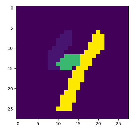
The text data I collected from the site included textual classifications of the product as well as its Amazon ID, title, and the highest and lowest prices it had achieved during the past year. Conveniently, those two price points allowed me to calibrate the y-axis of the price history graph image. I designed a method that would find the boundaries of the graph panel within the image, trace up the right-hand border pixel-by-pixel until it found the colored price line, and then trace that line from right to left across the image, jumping over gaps in price coverage as necessary. It did this separately for Amazon-sold items, third party new items, and third party used items (each had a different color in the graph). I wrote a function to edit the URL such that the graph image would display to an arbitrarily large size (an oversight, perhaps, by the folks at CamelCamelCamel), allowing me to achieve greater precision in my calibrations and obtain uniformly-sized graph images for each product.


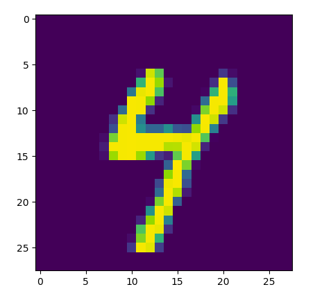
Example Graph (Amazon in green, 3rd party new in blue, 3rd party used in red):

Amazon example.png


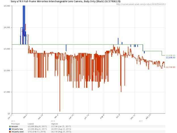
As I do not have access to the actual raw data, I have no way of performing conclusive error analysis, though I’ve recreated the graphs from the scraped price data and found that they overlap very consistently. As the maximum price and minimum price were used to calibrate the image, their error was expectedly quite low (within a rounding error). However, I was able to compare the most recent price in the scraped data to the most recent price visually imprinted in the graph image and found that they were within a dollar of each other for items costing a few hundred dollars (~0.5%), which should be sufficiently low for informative analysis.


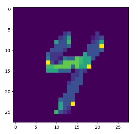
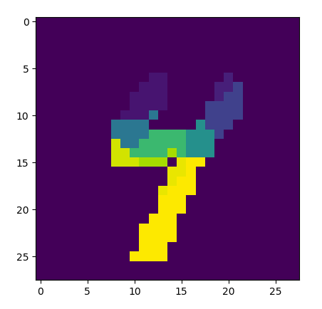
Example 3rd party used graph vs scraped results re-graphed:

This slideshow requires JavaScript.


Findings:

As a photography enthusiast, I couldn’t help but investigate one of the age-old questions in the photography community: Canon vs Nikon. Additionally, as a fan of Sony’s new Alpha series cameras (including the A7RII/III mirrorless line), I threw in Sony for comparison. How do prices and price volatility compare between these three large camera brands?


Amazon analysis price.png

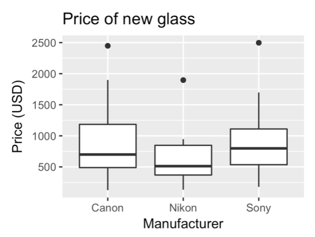
Sony has more expensive lenses on average, having made large strides into the mirrorless market recently.


Amazon analysis price drop 4 months.png

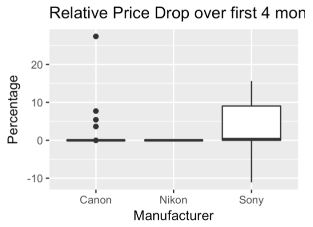
However, Sony has been expanding into the mirrorless market at a very aggressive pace, releasing more cameras in a year or two than Canon or Nikon may in a decade. Perhaps as a result of this, Sony’s cameras show a much faster price drop over the first four months than both Canon and Nikon cameras.


Amazon analysis mode - mean.png

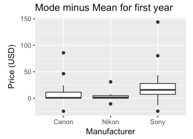
I tried to measure “flash sales” (i.e. sales that exist only for a very short period of time) using the mean price (which will be skewed by extreme values) subtracted from the mode price (which represents the “sitting” or standard/normal price of the items), and I found that Nikon has relatively stable prices (and Sony’s as expected, are the most volatile).


This slideshow requires JavaScript.

Sony’s prices also had a larger standard deviation within the third-party new and Amazon-sold categories, consistent with company sales. Canon’s prices showed a larger standard deviation in the third-party used market, perhaps showing that Canon users have a more active used gear market (which matches with personal anecdotal observations, for what it’s worth).


Although more analysis could easily be done, the point of such efforts is as a proof of concept that creative approaches to web scraping can yield data that are otherwise unaccessible.

A Brief Explanation of My Master’s Thesis

While impossible to cover the full breadth of the 204-page behemoth itself, for those curious I’ve included a computer science-only highlight summary of my Master’s thesis. I’m shying away from most bioscience terminology and avoiding most of the biological background, as the goal of this article is to overview my project for those outside the field.


Motivations:

Photosynthesis is incredibly important for life on Earth as we know it, as it creates and sustains the oxygen in the air that we breathe. Much of that oxygen is produced not only by plants (though they do play a large role) but by cyanobacteria (photosynthetic bacteria that also formed the foundation for how photosynthesis works in plants and algae) covering the world’s oceans. There are many basic biological questions about these essential creatures that we don’t understand. One involves how these life-giving membranes divide.


Analogy:

Cellular division is fairly well understood, but that’s only part of the puzzle of how such cells divide. If you imagine dividing a lasagna in two for two people to eat, you simply can’t separate the two halves without separating each layer from top to bottom; you have to make a full cross-sectional cut to separate the two pieces. Carrying this analogy forward, cellular division (division of the cellular membranes and the cells themselves) only handles how the top-most and bottom-most layers of the lasagna get cut—the inner layers (here, the thylakoid membranes) must also be split through some unknown mechanism.


Summary:

As a one-sentence summary of the thesis, I propose a short but comprehensive set of possibilities for how this (thylakoid membrane division) might occur, observe the process carefully in two divergent species of cyanobacteria using light microscopy, implement a new image segmentation technique tailored for this setup, and find that the two species appear to use different processes for dividing their thylakoid membranes, one orderly and one disorderly.


These findings suggest different approaches for discovering the mechanistic details of how this division occurs, and I lay the groundwork and a roadmap for future work in this area, including specifying possible genetic targets (though I’ll skip that here).


Figures:

Master's Thesis Wikipedia Synechocystis.png

General (simplified) thylakoid membrane morphology, using genus Synechocystis as example. Source: Wikimedia Commons.

Master's Thesis Models.png

Division models proposed in my thesis (the thylakoid membranes are shown in green with red edges). On the left we have division triggered specifically in advance of the dividing cell membranes; in the middle we have sufficiently frequent division such that a triggering mechanism is not needed; on the right we have no division mechanism short of the thylakoids being forcefully “cut” by the dividing cell membranes.


Burden Placed on Image Analysis:

The relevant details here are those relating to the segmentation algorithm I developed and implemented. A few background observations are also important to note. First, these bacteria are small and grow in clusters with very little distance to separate each individual cell. The combination of these two factors in particular makes proper segmentation of each cell difficult. Edges, that when observed at a large scale are sharp, are instead necessarily blurry due to the diffraction limit of light (the cells are not much larger than the waves we’re using to image them, so resolution is inherently limited by the physics of light). The high magnification required to visualize the cells (and their internal membranes) also means that we won’t be able to afford a high density of photons per pixel in the image, which means that the images will be inherently noisy (grainy) as well. Attempts to mitigate either of these problems (the blur and the noise) by choosing a smaller wavelength or increasing the intensity of light will poison the cyanobacteria with light outside their acceptable range of energies (the photosystems are tuned to specific frequencies within the orange-red part of the visual spectrum, and they can only sustain so much irradiative intensity before being damaged and destroyed). Longer exposures miss out on potentially important second-by-second information about the division process (yes, I did find significant movements that occurred faster than the framerate could capture) and are also not ideal. As such, we unfortunately have to manage these problems in silico (computationally) instead of in vivo (physically). Offloading these physical problems onto the computational side of the project places a high burden on the image analysis system. Typical tools used to segment images of cells (typically much larger, eukaryotic cells) performed poorly, often segmenting clusters of cells and/or mere portions of cells.


Imaging Solutions:

I implemented a dual-channel approach in which two related but independent measures of cell shape were taken: one using phase contrast and one using the inherent fluorescence of the thylakoid membranes distributed throughout the cells. Phase contrast microscopy uses differences in refractive index (specifically the retardation of light waves passing through media of higher refractive index) and the ability of light to self-interfere to bring attention to the borders between objects of different refractive index (in a physical as opposed to non-computational way). It is the standard approach for cell segmentation, but as indicated earlier, due to the difficulties of this particular imaging setup, it performed poorly on its own. Consecutive phase contrast images were also too correlated and mistakes made on one by the general segmentation software were often repeated on the other. Cyanobacteria, due specifically to their light-feeding properties, are also fluorescent under certain wavelengths of light. I imaged each field alternatingly in quick succession using phase contrast and epifluorescence microscopy (epifluorescence specifically measures light emitted by a fluorescent object, as opposed to possible reflections or diffractions around it). These two orthogonal (in the informational though not geometrical sense) measures of cell shape provided much more information for accurately segmenting the cells, so I went about implementing my own image segmentation algorithm capable of simultaneously using information from both channels.


The benefits of using these two imaging techniques go deeper than just providing alternate estimates of the cells’ shapes. Each has its own associated gradient, and these gradients properly anti-align at the cell boundary (thylakoid fluorescence is brightest inside the cell, where the thylakoids actually are, and phase contrast is darkest inside the cell, due to the cell contents’ slowing of light as it passes through leading to interference). The information gathered from each source therefore had the greatest detail (toward the right side of the histogram in photographer’s terms) where the other had the least detail (toward the left side of the histogram); the sources were exceptionally complementary.


Algorithmic Approach:

The use of these complementary imaging methods made it feasible to segment cells, but what about the greater task of segmenting some ten thousand frames of a hundred or more cells each within a reasonable time frame? One typical approach is to use constricting polygons around each cell center with an “energy” function that penalizes large distance between the vertices of the polygon and further penalizes sharp angles between polygon edges in a manner tunable with hyperparameters. Such methods calculate the total energy around the perimeter of the cell many times as a local energy minimum is approached. Such an approach, aside from being computationally expensive when considering a million cell-frames, is weak both to local minima in noisy images and to thin cells pressed side-by-side in clusters, both of which are characteristics of the imaging context we’re considering here. I knew a more appropriate method would be required, and set out to design one from scratch starting from first principles and immediately considering this unique imaging context.


The longer-term goals of the imaging project were to carefully and accurately analyze aspects of cell shape and internal thylakoid membrane shape throughout the division cycle, which would require exceptionally accurate estimations of cell size and (angular) orientation for spatial alignments and averaging across multiple cells (for seeing through the fog of noise in particular). I therefore decided to highly prioritize accuracy in segmented cell shape at the cost of “missing” some cell-frames (i.e. biasing towards type II-like errors—dropping a correct cell outline—for the sake of minimizing type I-like errors—wrongly accepting an incorrect outline), which could be compensated for by just averaging over even more data. I’d need to develop a fast algorithm, preferably analyzing each cell-frame’s cell outline just once, in order to capture enough data for the high degree of averaging I’d be doing.


The Algorithm:

I decided on a snake-like algorithm that would start from the most recognizably cell-edge-like pixel around a cell center and progress one circumference along the cell edge pixel-by-pixel. The direction of travel by the edge finder was guided orthogonally by both the thylakoid epifluorescence and phase contrast image gradients (following directions in which the direction’s cross product with each gradient had high magnitude and opposite sign) and also by the previous directions traveled (allowing movements in directions for which the dot product of current direction and average previous direction are non-negative). In this manner, the algorithm would analyze only a local window of pixels around each cell’s edge only once, and it would terminate once it formed a closed loop of reasonable perimeter and eccentricity with centroid sufficiently similar to the last capture (as quality control to maintain accurate cell outlines). Each overall frame was first thresholded (with binary openings to reduce noise) in each image channel to best find cell centers and define reasonable realms in which the snakes could roam (for instance, not allowing them to stray off too far from the cell clusters). I tuned hyperparameters for each species of cyanobacteria (one rod-shaped, one approximately spherical) to best apply strict quality control to acceptable cell outlines that were being tracked and analyzed.


Each cell was assigned a uniquely identifying number and tracked over its lifetime from first detection to division into two separately segmentable cells. The cells were physically held in place by their being sandwiched between the imaging glass (slide) and a nutrient-containing agarose hydrogel to prevent drift, and the algorithm would remember each cells’ centroid for continued tracking and update said centroid with subsequent frame in case of drift (which did occur—in sudden, earthquake-like fashion, though maximal drift only reached 1-2 pixels per frame—as the agarose hydrogel slowly dried over the 24+ hours of imaging).


Data (such as calculated centroid, angular orientation, eccentricity, length, width, etc.) on each cell in each frame was saved in a large array, and a local snapshot of the cell centered at the cell’s centroid (in both phase contrast and epifluorescence) was saved to a directory particular to each cell. After the full segmentation run was completed, each cell’s course of division could be viewed in video format by stitching together that cell’s snapshot (in either phase contrast or epifluorescence) in each frame, along with an optional temporal Gaussian blur (applied over a few consecutive frames with a stride of 1) for image clarity. Furthermore, a composite video was created for each image type (phase contrast or epifluorescence) and species showing an average time course of division for that species by spatially rotating each cell’s images by their orientation at that time and temporally aligning each cell’s snapshots in reference to the frame of its completion of division.


A Few Example Images:

This slideshow requires JavaScript.


Findings:

Aside from the aforementioned finding that one species’ thylakoid division process was orderly (appearing as a very clear, non-dynamic structure that would split along the division plane partway through cell division) and the other was disorderly (appearing as a highly dynamic set of constantly forming and breaking thylakoid connections between roaming thylakoid regions that seemed to make way for the dividing cell membranes on their own just through constantly rearranging), a few other results from the field were recapitulated. Cell division was found to be loosely synchronized in one species as previously reported and completely asynchronous in the other (also as previously reported).


Example of High-Throughput Analysis:

Master's Thesis Synechococcus data.png

Due to the significant amount of noise, analysis was only possible using high-throughput and highly averaged approaches (necessitating the image segmentation algorithm). Over one hundred distinct cells’ data (colored traces in the background) were averaged over their lifetimes (black trace in the foreground) to generate insights. Here we see potential evidence of thylakoid membrane division in advance of the completion of cell division in Synechococcus, supporting Model 1 for this species.


Discussion:

Overall, this process gave me a solid experience-based foundation in methods of image segmentation and image analysis generally, which I carry with me in my current work as a data scientist. According to a recent survey-based report by Kaggle, image data is the third-most common data type used in the field of data science, after relational data and textual data, and comprises an estimated one sixth of data science work (including video data). Based on personal experience, it also seems to be relatively ignored among data scientists in training, who generally stick to the less esoteric realm of relational and textual data. It’s given me a greater perspective on the overall process of finding kernels of truth within seas of information as well as a few translatable skills that I can cross-apply to data analysis tasks in general.

All About the Digits: Approaches to the Canonical MNIST Dataset

Links to code on Github: mnist_utils.py and mnist_features.py


Executive Summary:

I’ve created a set of functions that can pre-identify some features in the MNIST data set that one would normally imagine a first or second hidden layer handling. Mainly, it can identify (with some limited success) distinct straight line segments. Further steps will include feeding this information into a neural network to assess whether it improves classification accuracy or not, and improving the feature detection as well.


Motivations:

Neural networks, especially those of the convolutional or capsule variety, have an astounding ability to recognize and process images. However, they come with one major drawback: the reliance on an enormous volume of data for training. The amount of data and training they require is often a barrier to developing a competent network at a sufficiently difficult task (in terms of access to enough data or access to enough computing power). This need is beyond that of other machine learning approaches, and well beyond what seems necessary for learning in their distant biological cousins. For instance, I let you study one example of one Chinese character closely for some time (a few minutes should suffice), even with no prior knowledge of Chinese, you would be able to discern it against other Chinese characters. Furthermore, you would nearly as easily recognize it in scale- and rotationally variant forms. As deeper neural networks (which have traditionally been the direction for improving computer vision performance) explore increasingly astronomic possibility spaces (in which it’s hard to imagine converging on a workable solution), I can’t help but wonder if there are any sensible hard-coded features that are worth adding into neural networks to allow shallower neural networks (and accordingly less data and less processing) to achieve similar performance, as if by acting as a replacement solution for one or more lower layers. Such an approach would also help to make the resulting neural network systems less of a black box. Below, as an ongoing project, I’ve catalogued some explorations into possible features that may aid in classification of the MNIST handwritten digits, with the purpose of further improving my understanding of image techniques and as a means to explore neural networks.


The feature detection works by calculating basic image gradients at each pixel, arbitrarily assigning a direction orthogonal to the gradient at each pixel (always a ninety-degree rotation in the same direction), clustering the pixels into discrete groups based on pixel alignment with their neighbors, and systematically flipping the polarity of their directions until optimally “laminar” flow is achieved throughout the whole system (until each pixel group is most similarly aligned with its neighbor groups). These groups, when further clustered by similarity in alignment, outline distinct line segments.


Original image:

MNIST 4-1 raw.png

Angle based on gradient direction:

MNIST 4-1 gradient.png

Clustered into small groups:

MNIST 4-1 semi-joined.png

Joined into segments:

MNIST 4-1 joined.png


Below are two examples for each digit. Results are unfortunately still inconsistent for curvy digits (0, 2, 3, 5, 6, 8, 9), though fairly consistent for straighter-line digits (1, 4, and 7).